# Topics 3
## 1. Read replica pattern
In this post, we talk about a simple yet commonly used database design pattern (setup): Read replica pattern.
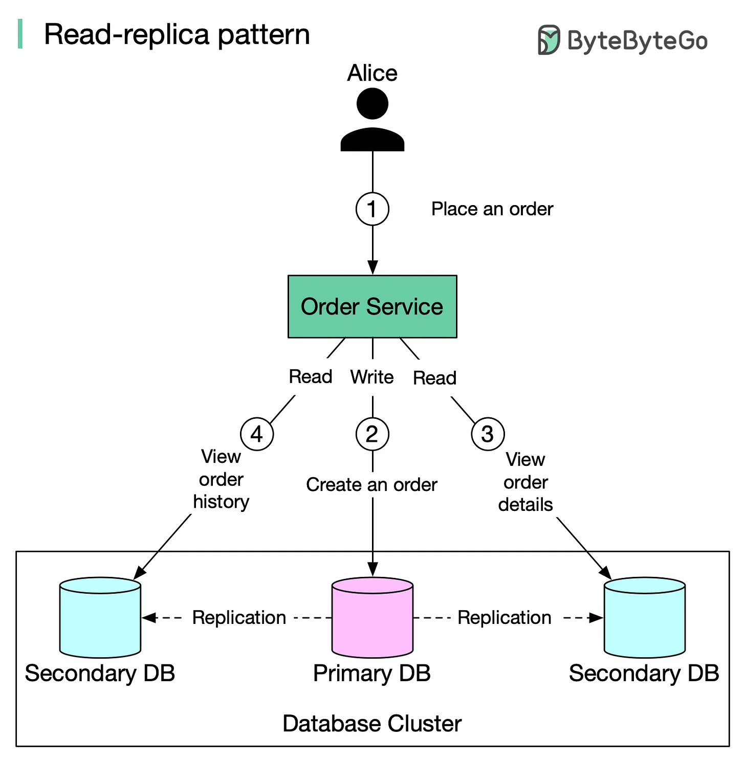
In this setup, all data-modifying commands like insert, delete, or update are sent to the primary DB and reads are sent to read replicas.
The diagram below illustrates the setup:
* When Alice places an order on amazon.com, the request is sent to Order Service.
* Order Service creates a record about the order in the primary DB (write). Data is replicated to two replicas.
* Alice views the order details. Data is served from a replica (read).
* Alice views the recent order history. Data is served from a replica (read).
There is one major problem in this setup: replication lag.
Under certain circumstances (network delay, server overload, etc.), data in replicas might be seconds or even minutes behind. In this case, if Alice immediately checks the order status (query is served by the replica) after the order is placed, she might not see the order at all. This leaves Alice confused. In this case, we need “read-after-write” consistency.
Possible solutions to mitigate this problem:
1️⃣ Latency sensitive reads are sent to the primary database.
2️⃣ Reads that immediately follow writes are routed to the primary database.
3️⃣ A relational DB generally provides a way to check if a replica is caught up with the primary. If data is up to date, query the replica. Otherwise fail the read request or read from the primary.
## 2. How to implement read replica pattern
There are two common ways to implement the read replica pattern:
1. Embed the routing logic in the application code (explained in the last post).
2. Use database middleware.
We focus on option 2 here. The middleware provides transparent routing between the application and database servers. We can customize the routing logic based on difficult rules such as user, schema, statement, etc.
The diagram below illustrates the setup:
1. When Alice places an order on amazon, the request is sent to Order Service.
2. Order Service does not directly interact with the database. Instead, it sends database queries to the database middleware.
3. The database middleware routes writes to the primary database. Data is replicated to two replicas.
4. Alice views the order details (read). The request is sent through the middleware.
5. Alice views the recent order history (read). The request is sent through the middleware.
The database middleware acts as a proxy between the application and databases. It uses standard MySQL network protocol for communication.
Pros:
* Simplified application code. The application doesn’t need to be aware of the database topology and manage access to the database directly.
* Better compatibility. The middleware uses the MySQL network protocol. Any MySQL compatible client can connect to the middleware easily. This makes database migration easier.
Cons:
* Increased system complexity. A database middleware is a complex system. Since all database queries go through the middleware, it usually requires a high availability setup to avoid a single point of failure.
* Additional middleware layer means additional network latency. Therefore, this layer requires excellent performance.
## 3. What happens when you type a URL into your browser?
What happens when you type a URL into your browser?
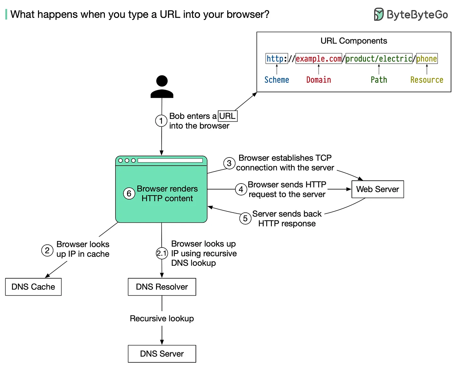
The diagram below illustrates the steps.
1. Bob enters a URL into the browser and hits Enter. In this example, the URL is composed of 4 parts:
🔹 scheme - http\://. This tells the browser to send a connection to the server using HTTP. 🔹 domain - example.com. This is the domain name of the site. 🔹 path - product/electric. It is the path on the server to the requested resource: phone. 🔹 resource - phone. It is the name of the resource Bob wants to visit.
2. The browser looks up the IP address for the domain with a domain name system (DNS) lookup. To make the lookup process fast, data is cached at different layers: browser cache, OS cache, local network cache, and ISP cache.
2.1 If the IP address cannot be found at any of the caches, the browser goes to DNS servers to do a recursive DNS lookup until the IP address is found (this will be covered in another post).
3. Now that we have the IP address of the server, the browser establishes a TCP connection with the server.
4. The browser sends an HTTP request to the server. The request looks like this:
𝘎𝘌𝘛 /𝘱𝘩𝘰𝘯𝘦 𝘏𝘛𝘛𝘗/1.1 𝘏𝘰𝘴𝘵: 𝘦𝘹𝘢𝘮𝘱𝘭𝘦.𝘤𝘰𝘮
5. The server processes the request and sends back the response. For a successful response (the status code is 200). The HTML response might look like this:
𝘏𝘛𝘛𝘗/1.1 200 𝘖𝘒 𝘋𝘢𝘵𝘦: 𝘚𝘶𝘯, 30 𝘑𝘢𝘯 2022 00:01:01 𝘎𝘔𝘛 𝘚𝘦𝘳𝘷𝘦𝘳: 𝘈𝘱𝘢𝘤𝘩𝘦 𝘊𝘰𝘯𝘵𝘦𝘯𝘵-𝘛𝘺𝘱𝘦: 𝘵𝘦𝘹𝘵/𝘩𝘵𝘮𝘭; 𝘤𝘩𝘢𝘳𝘴𝘦𝘵=𝘶𝘵𝘧-8
\ <𝘩𝘵𝘮𝘭 𝘭𝘢𝘯𝘨="𝘦𝘯"> 𝘏𝘦𝘭𝘭𝘰 𝘸𝘰𝘳𝘭𝘥 \
6. The browser renders the HTML content.
## 4. How does the Domain Name System (DNS) lookup work?
How does the Domain Name System (DNS) lookup work?
DNS acts as an address book. It translates human-readable domain names (google.com) to machine-readable IP addresses (142.251.46.238).
To achieve better scalability, the DNS servers are organized in a hierarchical tree structure.
There are 3 basic levels of DNS servers:
Root name server (.). It stores the IP addresses of Top Level Domain (TLD) name servers. There are 13 logical root name servers globally.
1. TLD name server. It stores the IP addresses of authoritative name servers. There are several types of TLD names. For example, generic TLD (.com, .org), country code TLD (.us), test TLD (.test).
2. Authoritative name server. It provides actual answers to the DNS query. You can register authoritative name servers with domain name registrar such as GoDaddy, Namecheap, etc.
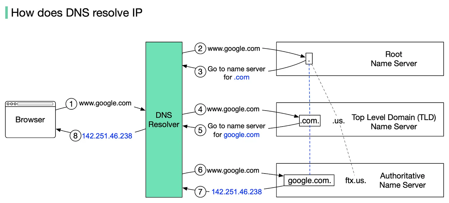
The diagram below illustrates how DNS lookup works under the hood:
1. google.com is typed into the browser, and the browser sends the domain name to the DNS resolver.
2. The resolver queries a DNS root name server.
3. The root server responds to the resolver with the address of a TLD DNS server. In this case, it is .com.
4. The resolver then makes a request to the .com TLD.
5. The TLD server responds with the IP address of the domain’s name server, google.com (authoritative name server).
6. The DNS resolver sends a query to the domain’s nameserver.
7. The IP address for google.com is then returned to the resolver from the nameserver.
8. The DNS resolver responds to the web browser with the IP address (142.251.46.238) of the domain requested initially.
DNS lookups on average take between 20-120 milliseconds to complete (according to YSlow).
## 5. Storage systems overview
In this post, let’s review the storage systems in general.
Storage systems fall into three broad categories:
🔹 Block storage
🔹 File storage
🔹 Object storage
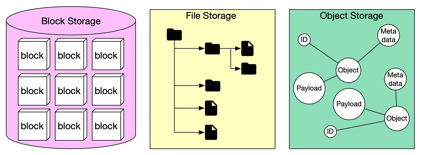
The diagram below illustrates the comparison of different storage systems.
Block Storage
Block storage came first, in the 1960s. Common storage devices like hard disk drives (HDD) and solid-state drives (SSD) that are physically attached to servers are all considered as block storage.
Block storage presents the raw blocks to the server as a volume. This is the most flexible and versatile form of storage. The server can format the raw blocks and use them as a file system, or it can hand control of those blocks to an application. Some applications like a database or a virtual machine engine manage these blocks directly in order to squeeze every drop of performance out of them.
Block storage is not limited to physically attached storage. Block storage could be connected to a server over a high-speed network or over industry-standard connectivity protocols like Fibre Channel (FC) and iSCSI. Conceptually, the network-attached block storage still presents raw blocks. To the servers, it works the same as physically attached block storage. Whether to a network or physically attached, block storage is fully owned by a single server. It is not a shared resource.
File storage
File storage is built on top of block storage. It provides a higher-level abstraction to make it easier to handle files and directories. Data is stored as files under a hierarchical directory structure. File storage is the most common general-purpose storage solution. File storage could be made accessible by a large number of servers using common file-level network protocols like SMB/CIFS and NFS. The servers accessing file storage do not need to deal with the complexity of managing the blocks, formatting volume, etc. The simplicity of file storage makes it a great solution for sharing a large number of files and folders within an organization.
Object storage
Object storage is new. It makes a very deliberate tradeoff to sacrifice performance for high durability, vast scale, and low cost. It targets relatively “cold” data and is mainly used for archival and backup. Object storage stores all data as objects in a flat structure. There is no hierarchical directory structure. Data access is normally provided via a RESTful API. It is relatively slow compared to other storage types. Most public cloud service providers have an object storage offering, such as AWS S3, Google block storage, and Azure blob storage.
## 6. S3-like storage system
What happens when you upload a file to Amazon S3?
Before we dive into the design, let’s define some terms.
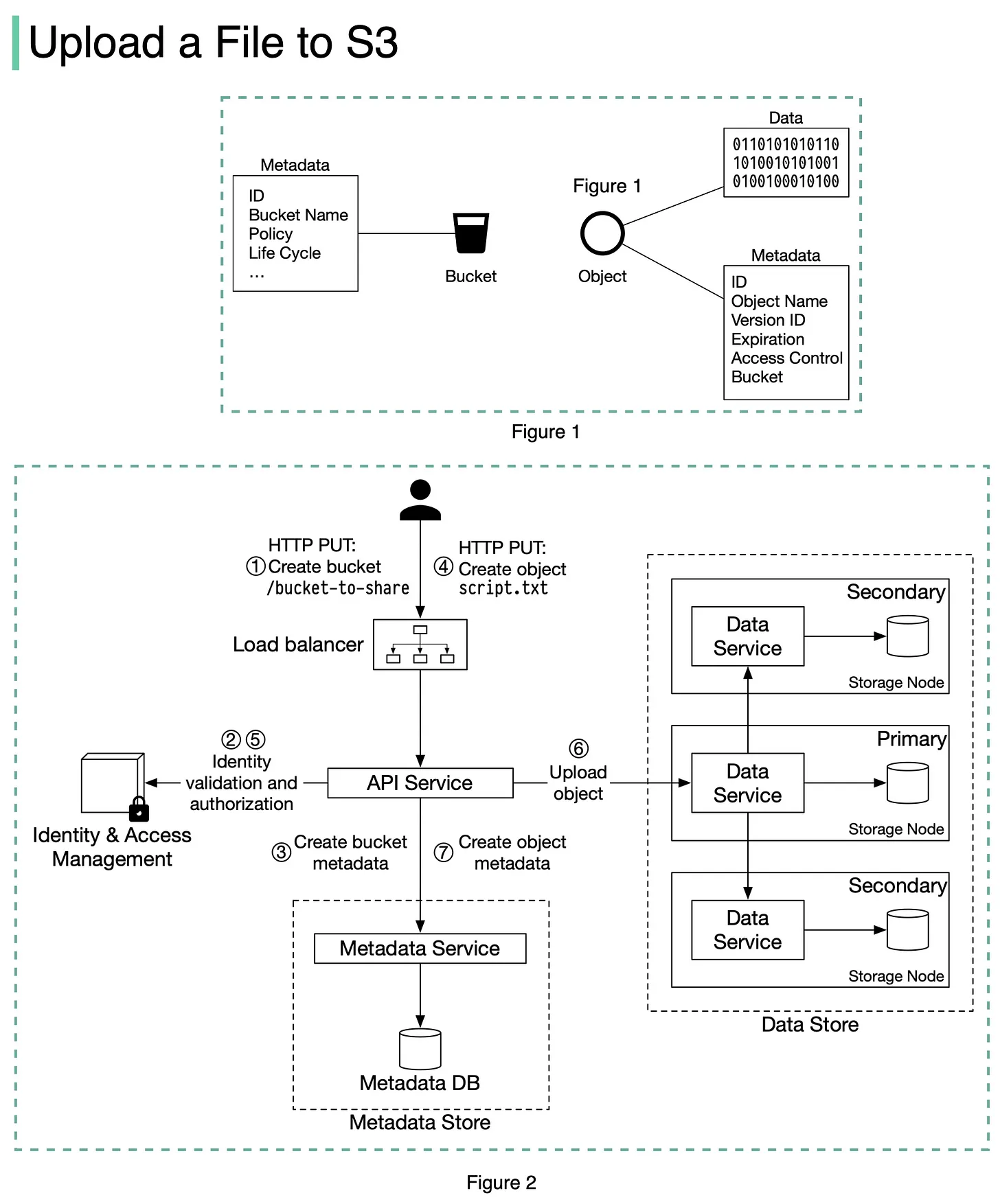
𝐁𝐮𝐜𝐤𝐞𝐭. A logical container for objects. The bucket name is globally unique. To upload data to S3, we must first create a bucket.
𝐎𝐛𝐣𝐞𝐜𝐭. An object is an individual piece of data we store in a bucket. It contains object data (also called payload) and metadata. Object data can be any sequence of bytes we want to store. The metadata is a set of name-value pairs that describe the object.
An S3 object consists of (Figure 1): 🔹 Metadata. It is mutable and contains attributes such as ID, bucket name, object name, etc. 🔹 Object data. It is immutable and contains the actual data.
In S3, an object resides in a bucket. The path looks like this: /bucket-to-share/script.txt. The bucket only has metadata. The object has metadata and the actual data.
The diagram below (Figure 2) illustrates how file uploading works. In this example, we first create a bucket named “bucket-to-share” and then upload a file named “script.txt” to the bucket.
1. The client sends an HTTP PUT request to create a bucket named “bucket-to-share.” The request is forwarded to the API service.
2. The API service calls Identity and Access Management (IAM) to ensure the user is authorized and has WRITE permission.
3. The API service calls the metadata store to create an entry with the bucket info in the metadata database. Once the entry is created, a success message is returned to the client.
4. After the bucket is created, the client sends an HTTP PUT request to create an object named “script.txt”.
5. The API service verifies the user’s identity and ensures the user has WRITE permission on the bucket.
6. Once validation succeeds, the API service sends the object data in the HTTP PUT payload to the data store. The data store persists the payload as an object and returns the UUID of the object.
7. The API service calls the metadata store to create a new entry in the metadata database. It contains important metadata such as the object\_id (UUID), bucket\_id (which bucket the object belongs to), object\_name, etc.
## 7. How does foreign exchange work from the system's perspective?
Have you wondered what happens under the hood when you pay with USD and the seller from Europe receives EUR (euro)? This process is called foreign exchange.
Suppose Bob (the buyer) needs to pay 100 USD to Alice (the seller), and Alice can only receive EUR. The diagram below illustrates the process.
1. Bob sends 100 USD via a third-party payment provider. In our example, it is Paypal. The money is transferred from Bob’s bank account (Bank B) to Paypal’s account in Bank P1.
2. Paypal needs to convert USD to EUR. It leverages the foreign exchange provider (Bank E). Paypal sends 100 USD to its USD account in Bank E.
3. 100 USD is sold to Bank E’s funding pool.
4. Bank E’s funding pool provides 88 EUR in exchange for 100 USD. The money is put into Paypal’s EUR account in Bank E.
5. Paypal’s EUR account in Bank P2 receives 88 EUR.
6. 88 EUR is paid to Alice’s EUR account in Bank A.
Now let’s take a close look at the foreign exchange (forex) market. It has 3 layers:
🔹 Retail market. Funding pools are parts of the retail market. To improve efficiency, Paypal usually buys a certain amount of foreign currencies in advance. 🔹 Wholesale market. The wholesale business is composed of investment banks, commercial banks, and foreign exchange providers. It usually handles accumulated orders from the retail market. 🔹 Top-level participants. They are multinational commercial banks that hold lots of money from different countries.
When Bank E’s funding pool needs more EUR, it goes upward to the wholesale market to sell USD and buy EUR. When the wholesale market accumulates enough orders, it goes upward to top-level participants. Steps 3.1-3.3 and 4.1-4.3 explain how it works.
## 8. Erasure coding
A really cool technique that’s commonly used in object storage such as S3 to improve durability is called erasure coding. Let’s take a look at how it works.
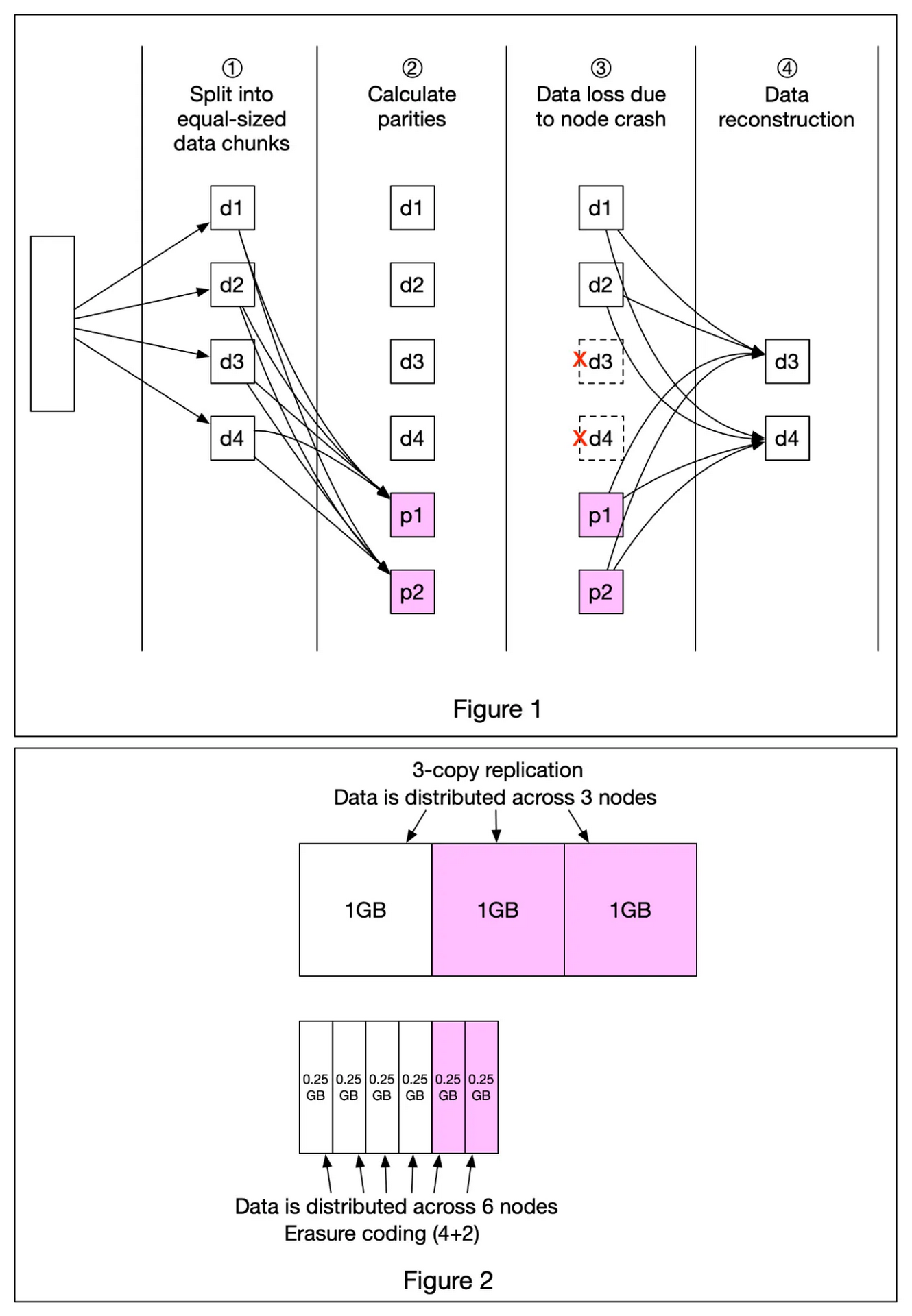
Erasure coding deals with data durability differently from replication. It chunks data into smaller pieces (placed on different servers) and creates parities for redundancy. In the event of failures, we can use chunk data and parities to reconstruct the data. Let’s take a look at a concrete example (4 + 2 erasure coding) as shown in Figure 1.
1️⃣ Data is broken up into four even-sized data chunks d1, d2, d3, and d4.
2️⃣ The mathematical formula is used to calculate the parities p1 and p2. To give a much simplified example, p1 = d1 + 2*d2 - d3 + 4*d4 and p2 = -d1 + 5*d2 + d3 - 3*d4.
3️⃣ Data d3 and d4 are lost due to node crashes.
4️⃣ The mathematical formula is used to reconstruct lost data d3 and d4, using the known values of d1, d2, p1, and p2.
How much extra space does erasure coding need? For every two chunks of data, we need one parity block, so the storage overhead is 50% (Figure 2). While in 3-copy replication, the storage overhead is 200% (Figure 2).
Does erasure coding increase data durability? Let’s assume a node has a 0.81% annual failure rate. According to the calculation done by Backblaze, erasure coding can achieve 11 nines durability vs 3-copy replication can achieve 6 nines durability.
## 9. How does CDN work?
A content delivery network (CDN) refers to geographically distributed servers (also called edge servers) that provide fast delivery of static and dynamic content. Let’s take a look at how it works.
Suppose Bob who lives in New York wants to visit an eCommerce website that is deployed in London. If the request goes to servers located in London, the response will be quite slow. So we deploy CDN servers close to where Bob lives, and the content will be loaded from the nearby CDN server.
The diagram below illustrates the process:
1. Bob types in [www.myshop.com](http://www.myshop.com) in the browser. The browser looks up the domain name in the local DNS cache.
2. If the domain name does not exist in the local DNS cache, the browser goes to the DNS resolver to resolve the name. The DNS resolver usually sits in the Internet Service Provider (ISP).
3. The DNS resolver recursively resolves the domain name (see my previous post for details). Finally, it asks the authoritative name server to resolve the domain name.
4. If we don’t use CDN, the authoritative name server returns the IP address for [www.myshop.com](http://www.myshop.com). But with CDN, the authoritative name server has an alias pointing to [www.myshop.cdn.com](http://www.myshop.cdn.com) (the domain name of the CDN server).
5. The DNS resolver asks the authoritative name server to resolve [www.myshop.cdn.com](http://www.myshop.cdn.com).
6. The authoritative name server returns the domain name for the load balancer of CDN [www.myshop.lb.com](http://www.myshop.lb.com).
7. The DNS resolver asks the CDN load balancer to resolve [www.myshop.lb.com](http://www.myshop.lb.com). The load balancer chooses an optimal CDN edge server based on the user’s IP address, user’s ISP, the content requested, and the server load.
8. The CDN load balancer returns the CDN edge server’s IP address for [www.myshop.lb.com](http://www.myshop.lb.com).
9. Now we finally get the actual IP address to visit. The DNS resolver returns the IP address to the browser.
10. The browser visits the CDN edge server to load the content. There are two types of contents cached on the CDN servers: static contents and dynamic contents. The former contains static pages, pictures, videos; the latter one includes results of edge computing.
11. If the edge CDN server cache doesn't contain the content, it goes upward to the regional CDN server. If the content is still not found, it will go upward to the central CDN server, or even go to the origin - the London web server. This is called the CDN distribution network, where the servers are deployed geographically.
## 10. Vertical partitioning vs horizontal partitioning
In many large-scale applications, data is divided into partitions that can be accessed separately. There are two typical strategies for partitioning data.
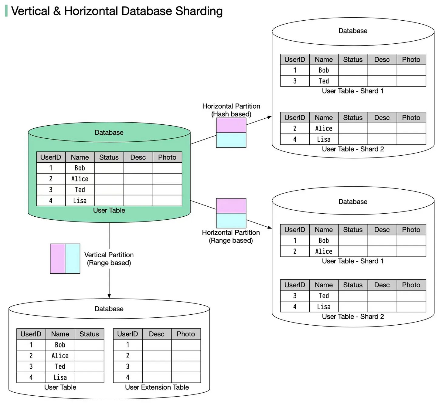
🔹 Vertical partitioning: it means some columns are moved to new tables. Each table contains the same number of rows but fewer columns (see diagram below).
🔹 Horizontal partitioning (often called sharding): it divides a table into multiple smaller tables. Each table is a separate data store, and it contains the same number of columns, but fewer rows (see diagram below).
Horizontal partitioning is widely used so let’s take a closer look.
Routing algorithm The routing algorithm decides which partition (shard) stores the data.
🔹 Range-based sharding. This algorithm uses ordered columns, such as integers, longs, timestamps, to separate the rows. For example, the diagram below uses the User ID column for range partition: User IDs 1 and 2 are in shard 1, User IDs 3 and 4 are in shard 2.
🔹 Hash-based sharding. This algorithm applies a hash function to one column or several columns to decide which row goes to which table. For example, the diagram below uses User ID mod 2 as a hash function. User IDs 1 and 3 are in shard 1, User IDs 2 and 4 are in shard 2.
Benefits 🔹 Facilitate horizontal scaling. Sharding facilitates the possibility of adding more machines to spread out the load.
🔹 Shorten response time. By sharding one table into multiple tables, queries go over fewer rows, and results are returned much more quickly.
Drawbacks 🔹 The order by operation is more complicated. Usually, we need to fetch data from different shards and sort the data in the application's code.
🔹 Uneven distribution. Some shards may contain more data than others (this is also called the hotspot).